9. LLN and CLT#
Contents
9.1. Overview#
This lecture illustrates two of the most important theorems of probability and statistics: The law of large numbers (LLN) and the central limit theorem (CLT).
These beautiful theorems lie behind many of the most fundamental results in econometrics and quantitative economic modeling.
The lecture is based around simulations that show the LLN and CLT in action.
We also demonstrate how the LLN and CLT break down when the assumptions they are based on do not hold.
In addition, we examine several useful extensions of the classical theorems, such as
The delta method, for smooth functions of random variables, and
the multivariate case.
Some of these extensions are presented as exercises.
We’ll need the following imports:
import matplotlib.pyplot as plt
plt.rcParams["figure.figsize"] = (11, 5)  #set default figure size
import random
import numpy as np
from scipy.stats import t, beta, lognorm, expon, gamma, uniform
from scipy.stats import gaussian_kde, poisson, binom, norm, chi2
from mpl_toolkits.mplot3d import Axes3D
from matplotlib.collections import PolyCollection
from scipy.linalg import inv, sqrtm
9.2. Relationships#
The CLT refines the LLN.
The LLN gives conditions under which sample moments converge to population moments as sample size increases.
The CLT provides information about the rate at which sample moments converge to population moments as sample size increases.
9.3. LLN#
We begin with the law of large numbers, which tells us when sample averages will converge to their population means.
9.3.1. The Classical LLN#
The classical law of large numbers concerns independent and identically distributed (IID) random variables.
Here is the strongest version of the classical LLN, known as Kolmogorov’s strong law.
Let
When it exists, let
In addition, let
Kolmogorov’s strong law states that, if
What does this last expression mean?
Let’s think about it from a simulation perspective, imagining for a moment that our computer can generate perfect random samples (which of course it can’t).
Let’s also imagine that we can generate infinite sequences so that the
statement
In this setting, (9.1) should be interpreted as meaning that the
probability of the computer producing a sequence where
9.3.2. Proof#
The proof of Kolmogorov’s strong law is nontrivial – see, for example, theorem 8.3.5 of [Dudley, 2002].
On the other hand, we can prove a weaker version of the LLN very easily and still get most of the intuition.
The version we prove is as follows: If
(This version is weaker because we claim only convergence in probability rather than almost sure convergence, and assume a finite second moment)
To see that this is so, fix
Recall the Chebyshev inequality, which tells us that
Now observe that
Here the crucial step is at the third equality, which follows from independence.
Independence means that if
As a result,
Combining our last result with (9.3), we come to the estimate
The claim in (9.2) is now clear.
Of course, if the sequence
While this doesn’t mean that the same line of argument is impossible, it does mean that if we want a similar result then the covariances should be “almost zero” for “most” of these terms.
In a long sequence, this would be true if, for example,
In other words, the LLN can still work if the sequence
This idea is very important in time series analysis, and we’ll come across it again soon enough.
9.3.3. Illustration#
Let’s now illustrate the classical IID law of large numbers using simulation.
In particular, we aim to generate some sequences of IID random variables and plot the evolution
of
Below is a figure that does just this (as usual, you can click on it to expand it).
It shows IID observations from three different distributions and plots
The dots represent the underlying observations
In each of the three cases, convergence of
n = 100

# Arbitrary collection of distributions
distributions = {"student's t with 10 degrees of freedom": t(10),
                 "β(2, 2)": beta(2, 2),
                 "lognormal LN(0, 1/2)": lognorm(0.5),
                 "γ(5, 1/2)": gamma(5, scale=2),
                 "poisson(4)": poisson(4),
                 "exponential with λ = 1": expon(1)}

# Create a figure and some axes
num_plots = 3
fig, axes = plt.subplots(num_plots, 1, figsize=(10, 20))

# Set some plotting parameters to improve layout
bbox = (0., 1.02, 1., .102)
legend_args = {'ncol': 2,
               'bbox_to_anchor': bbox,
               'loc': 3,
               'mode': 'expand'}
plt.subplots_adjust(hspace=0.5)

for ax in axes:
    # Choose a randomly selected distribution
    name = random.choice(list(distributions.keys()))
    distribution = distributions.pop(name)

    # Generate n draws from the distribution
    data = distribution.rvs(n)

    # Compute sample mean at each n
    sample_mean = np.empty(n)
    for i in range(n):
        sample_mean[i] = np.mean(data[:i+1])

    # Plot
    ax.plot(list(range(n)), data, 'o', color='grey', alpha=0.5)
    axlabel = '$\\bar{X}_n$ for $X_i \sim$' + name
    ax.plot(list(range(n)), sample_mean, 'g-', lw=3, alpha=0.6, label=axlabel)
    m = distribution.mean()
    ax.plot(list(range(n)), [m] * n, 'k--', lw=1.5, label=r'$\mu$')
    ax.vlines(list(range(n)), m, data, lw=0.2)
    ax.legend(**legend_args, fontsize=12)

plt.show()
<>:38: SyntaxWarning: invalid escape sequence '\s'
<>:38: SyntaxWarning: invalid escape sequence '\s'
/tmp/ipykernel_31715/2987866577.py:38: SyntaxWarning: invalid escape sequence '\s'
  axlabel = '$\\bar{X}_n$ for $X_i \sim$' + name
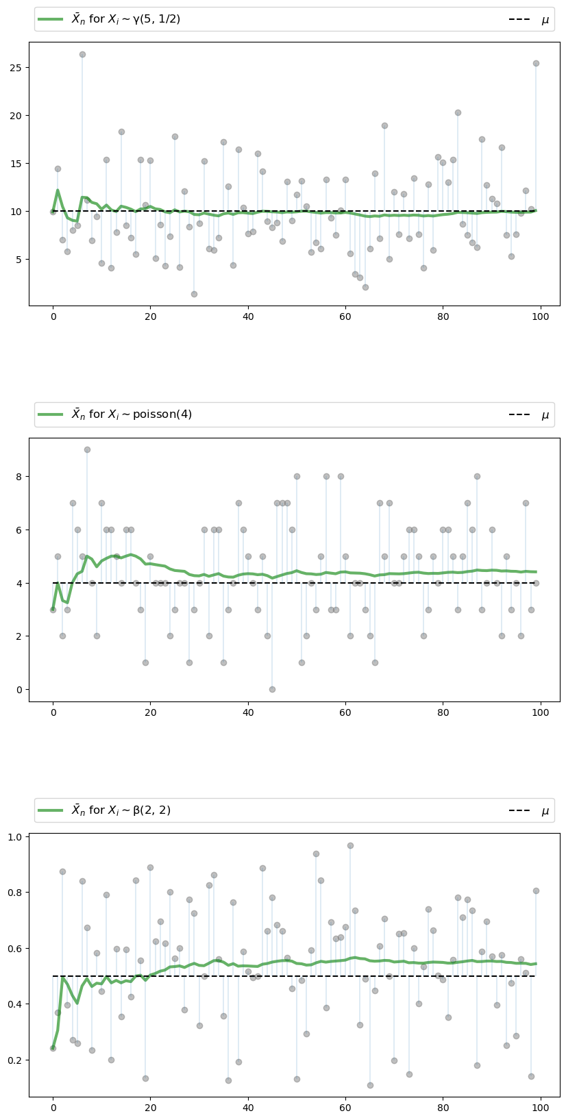
The three distributions are chosen at random from a selection stored in the dictionary distributions.
9.4. CLT#
Next, we turn to the central limit theorem, which tells us about the distribution of the deviation between sample averages and population means.
9.4.1. Statement of the Theorem#
The central limit theorem is one of the most remarkable results in all of mathematics.
In the classical IID setting, it tells us the following:
If the sequence
Here
9.4.2. Intuition#
The striking implication of the CLT is that for any distribution with finite second moment, the simple operation of adding independent copies always leads to a Gaussian curve.
A relatively simple proof of the central limit theorem can be obtained by working with characteristic functions (see, e.g., theorem 9.5.6 of [Dudley, 2002]).
The proof is elegant but almost anticlimactic, and it provides surprisingly little intuition.
In fact, all of the proofs of the CLT that we know are similar in this respect.
Why does adding independent copies produce a bell-shaped distribution?
Part of the answer can be obtained by investigating the addition of independent Bernoulli random variables.
In particular, let
Think of
The next figure plots the probability mass function of
fig, axes = plt.subplots(2, 2, figsize=(10, 6))
plt.subplots_adjust(hspace=0.4)
axes = axes.flatten()
ns = [1, 2, 4, 8]
dom = list(range(9))

for ax, n in zip(axes, ns):
    b = binom(n, 0.5)
    ax.bar(dom, b.pmf(dom), alpha=0.6, align='center')
    ax.set(xlim=(-0.5, 8.5), ylim=(0, 0.55),
           xticks=list(range(9)), yticks=(0, 0.2, 0.4),
           title=f'$n = {n}$')

plt.show()
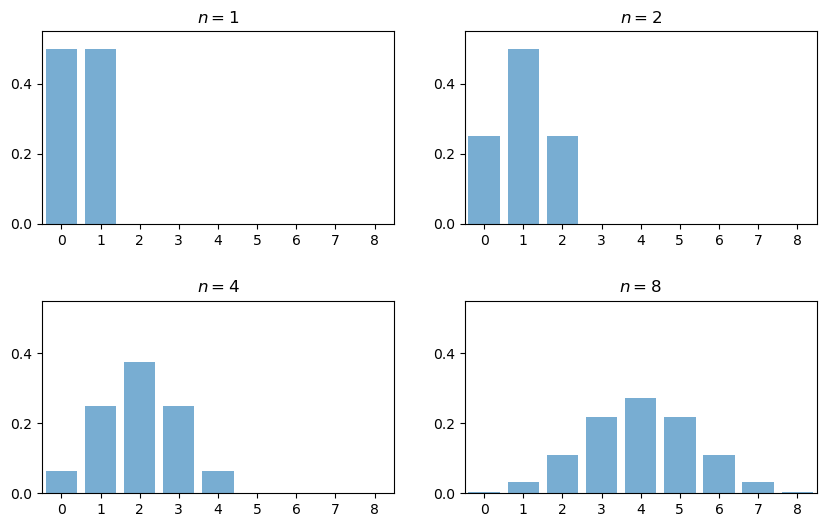
When
When
Notice the peak in probability mass at the mid-point
The reason is that there are more ways to get 1 success (“fail then succeed” or “succeed then fail”) than to get zero or two successes.
Moreover, the two trials are independent, so the outcomes “fail then succeed” and “succeed then fail” are just as likely as the outcomes “fail then fail” and “succeed then succeed”.
(If there was positive correlation, say, then “succeed then fail” would be less likely than “succeed then succeed”)
Here, already we have the essence of the CLT: addition under independence leads probability mass to pile up in the middle and thin out at the tails.
For
The intuition is the same — there are simply more ways to get these middle outcomes.
If we continue, the bell-shaped curve becomes even more pronounced.
We are witnessing the binomial approximation of the normal distribution.
9.4.3. Simulation 1#
Since the CLT seems almost magical, running simulations that verify its implications is one good way to build intuition.
To this end, we now perform the following simulation
Choose an arbitrary distribution
Generate independent draws of
Use these draws to compute some measure of their distribution — such as a histogram.
Compare the latter to
Here’s some code that does exactly this for the exponential distribution
(Please experiment with other choices of
# Set parameters
n = 250                  # Choice of n
k = 100000               # Number of draws of Y_n
distribution = expon(2)  # Exponential distribution, λ = 1/2
μ, s = distribution.mean(), distribution.std()

# Draw underlying RVs. Each row contains a draw of X_1,..,X_n
data = distribution.rvs((k, n))
# Compute mean of each row, producing k draws of \bar X_n
sample_means = data.mean(axis=1)
# Generate observations of Y_n
Y = np.sqrt(n) * (sample_means - μ)

# Plot
fig, ax = plt.subplots(figsize=(10, 6))
xmin, xmax = -3 * s, 3 * s
ax.set_xlim(xmin, xmax)
ax.hist(Y, bins=60, alpha=0.5, density=True)
xgrid = np.linspace(xmin, xmax, 200)
ax.plot(xgrid, norm.pdf(xgrid, scale=s), 'k-', lw=2, label=r'$N(0, \sigma^2)$')
ax.legend()

plt.show()
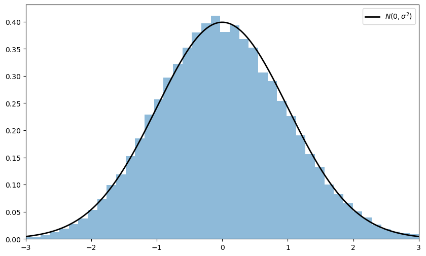
Notice the absence of for loops — every operation is vectorized, meaning that the major calculations are all shifted to highly optimized C code.
The fit to the normal density is already tight and can be further improved by increasing n.
You can also experiment with other specifications of
9.4.4. Simulation 2#
Our next simulation is somewhat like the first, except that we aim to track the distribution of
In the simulation, we’ll be working with random variables having
Thus, when
For
What we expect is that, regardless of the distribution of the underlying
random variable, the distribution of
The next figure shows this process for
(Taking a convex combination is an easy way to produce an irregular shape for
In the figure, the closest density is that of
beta_dist = beta(2, 2)

def gen_x_draws(k):
    """
    Returns a flat array containing k independent draws from the
    distribution of X, the underlying random variable.  This distribution
    is itself a convex combination of three beta distributions.
    """
    bdraws = beta_dist.rvs((3, k))
    # Transform rows, so each represents a different distribution
    bdraws[0, :] -= 0.5
    bdraws[1, :] += 0.6
    bdraws[2, :] -= 1.1
    # Set X[i] = bdraws[j, i], where j is a random draw from {0, 1, 2}
    js = np.random.randint(0, 2, size=k)
    X = bdraws[js, np.arange(k)]
    # Rescale, so that the random variable is zero mean
    m, sigma = X.mean(), X.std()
    return (X - m) / sigma

nmax = 5
reps = 100000
ns = list(range(1, nmax + 1))

# Form a matrix Z such that each column is reps independent draws of X
Z = np.empty((reps, nmax))
for i in range(nmax):
    Z[:, i] = gen_x_draws(reps)
# Take cumulative sum across columns
S = Z.cumsum(axis=1)
# Multiply j-th column by sqrt j
Y = (1 / np.sqrt(ns)) * S

# Plot
ax = plt.figure(figsize = (10, 6)).add_subplot(projection='3d')

a, b = -3, 3
gs = 100
xs = np.linspace(a, b, gs)

# Build verts
greys = np.linspace(0.3, 0.7, nmax)
verts = []
for n in ns:
    density = gaussian_kde(Y[:, n-1])
    ys = density(xs)
    verts.append(list(zip(xs, ys)))

poly = PolyCollection(verts, facecolors=[str(g) for g in greys])
poly.set_alpha(0.85)
ax.add_collection3d(poly, zs=ns, zdir='x')

ax.set(xlim3d=(1, nmax), xticks=(ns), ylabel='$Y_n$', zlabel='$p(y_n)$',
       xlabel=("n"), yticks=((-3, 0, 3)), ylim3d=(a, b),
       zlim3d=(0, 0.4), zticks=((0.2, 0.4)))
ax.invert_xaxis()
# Rotates the plot 30 deg on z axis and 45 deg on x axis
ax.view_init(30, 45)
plt.show()
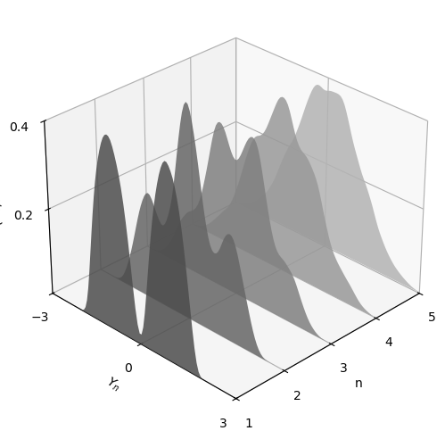
As expected, the distribution smooths out into a bell curve as
We leave you to investigate its contents if you wish to know more.
If you run the file from the ordinary IPython shell, the figure should pop up in a window that you can rotate with your mouse, giving different views on the density sequence.
9.4.5. The Multivariate Case#
The law of large numbers and central limit theorem work just as nicely in multidimensional settings.
To state the results, let’s recall some elementary facts about random vectors.
A random vector
Each realization of
A collection of random vectors
(The vector inequality
Let
The expectation
The variance-covariance matrix of random vector
Expanding this out, we get
The
With this notation, we can proceed to the multivariate LLN and CLT.
Let
Let
Interpreting vector addition and scalar multiplication in the usual way (i.e., pointwise), let
In this setting, the LLN tells us that
Here
The CLT tells us that, provided
9.5. Exercises#
Exercise 9.1
One very useful consequence of the central limit theorem is as follows.
Assume the conditions of the CLT as stated above.
If
This theorem is used frequently in statistics to obtain the asymptotic distribution of estimators — many of which can be expressed as functions of sample means.
(These kinds of results are often said to use the “delta method”.)
The proof is based on a Taylor expansion of
Taking the result as given, let the distribution
Derive the asymptotic distribution of
What happens when you replace
What is the source of the problem?
Solution to Exercise 9.1
Here is one solution
"""
Illustrates the delta method, a consequence of the central limit theorem.
"""

# Set parameters
n = 250
replications = 100000
distribution = uniform(loc=0, scale=(np.pi / 2))
μ, s = distribution.mean(), distribution.std()

g = np.sin
g_prime = np.cos

# Generate obs of sqrt{n} (g(X_n) - g(μ))
data = distribution.rvs((replications, n))
sample_means = data.mean(axis=1)  # Compute mean of each row
error_obs = np.sqrt(n) * (g(sample_means) - g(μ))

# Plot
asymptotic_sd = g_prime(μ) * s
fig, ax = plt.subplots(figsize=(10, 6))
xmin = -3 * g_prime(μ) * s
xmax = -xmin
ax.set_xlim(xmin, xmax)
ax.hist(error_obs, bins=60, alpha=0.5, density=True)
xgrid = np.linspace(xmin, xmax, 200)
lb = "$N(0, g'(\mu)^2  \sigma^2)$"
ax.plot(xgrid, norm.pdf(xgrid, scale=asymptotic_sd), 'k-', lw=2, label=lb)
ax.legend()
plt.show()
<>:27: SyntaxWarning: invalid escape sequence '\m'
<>:27: SyntaxWarning: invalid escape sequence '\m'
/tmp/ipykernel_31715/3132190149.py:27: SyntaxWarning: invalid escape sequence '\m'
  lb = "$N(0, g'(\mu)^2  \sigma^2)$"

What happens when you replace
In this case, the mean
Hence the conditions of the delta theorem are not satisfied.
Exercise 9.2
Here’s a result that’s often used in developing statistical tests, and is connected to the multivariate central limit theorem.
If you study econometric theory, you will see this result used again and again.
Assume the setting of the multivariate CLT discussed above, so that
The convergence
is valid.
In a statistical setting, one often wants the right-hand side to be standard normal so that confidence intervals are easily computed.
This normalization can be achieved on the basis of three observations.
First, if
Second, by the continuous mapping theorem, if
Third, if
Here
Putting these things together, your first exercise is to show that if
Applying the continuous mapping theorem one more time tells us that
Given the distribution of
where
(Recall that
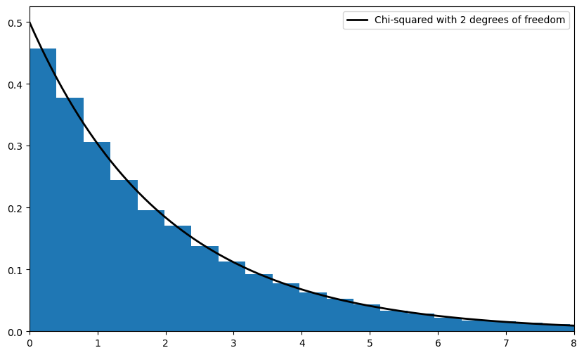
Your second exercise is to illustrate the convergence in (9.10) with a simulation.
In doing so, let
where
each
each
Hint
scipy.linalg.sqrtm(A)computes the square root ofA. You still need to invert it.You should be able to work out
Solution to Exercise 9.2
First we want to verify the claim that
This is straightforward given the facts presented in the exercise.
Let
By the multivariate CLT and the continuous mapping theorem, we have
Since linear combinations of normal random variables are normal, the
vector
Its mean is clearly
In conclusion,
Now we turn to the simulation exercise.
Our solution is as follows
# Set parameters
n = 250
replications = 50000
dw = uniform(loc=-1, scale=2)  # Uniform(-1, 1)
du = uniform(loc=-2, scale=4)  # Uniform(-2, 2)
sw, su = dw.std(), du.std()
vw, vu = sw**2, su**2
Σ = ((vw, vw), (vw, vw + vu))
Σ = np.array(Σ)

# Compute Σ^{-1/2}
Q = inv(sqrtm(Σ))

# Generate observations of the normalized sample mean
error_obs = np.empty((2, replications))
for i in range(replications):
    # Generate one sequence of bivariate shocks
    X = np.empty((2, n))
    W = dw.rvs(n)
    U = du.rvs(n)
    # Construct the n observations of the random vector
    X[0, :] = W
    X[1, :] = W + U
    # Construct the i-th observation of Y_n
    error_obs[:, i] = np.sqrt(n) * X.mean(axis=1)

# Premultiply by Q and then take the squared norm
temp = Q @ error_obs
chisq_obs = np.sum(temp**2, axis=0)

# Plot
fig, ax = plt.subplots(figsize=(10, 6))
xmax = 8
ax.set_xlim(0, xmax)
xgrid = np.linspace(0, xmax, 200)
lb = "Chi-squared with 2 degrees of freedom"
ax.plot(xgrid, chi2.pdf(xgrid, 2), 'k-', lw=2, label=lb)
ax.legend()
ax.hist(chisq_obs, bins=50, density=True)
plt.show()